Poisson Distribution

Suppose you work at a call center, approximately how many calls do you get in a day? It can be any number. Now, the entire number of calls at a call center in a day is modeled by Poisson distribution. Some more examples are

1. The number of emergency calls recorded at a hospital in a day.
2. The number of thefts reported in an area on a day.
3. The number of customers arriving at a salon in an hour.
4. The number of suicides reported in a particular city.
5. The number of printing errors at each page of the book.

You can now think of many examples following the same course. Poisson Distribution is applicable in situations where events occur at random points of time and space wherein our interest lies only in the number of occurrences of the event.

A distribution is called Poisson distribution when the following assumptions are valid:

1. Any successful event should not influence the outcome of another successful event.
2. The probability of success over a short interval must equal the probability of success over a longer interval.
3. The probability of success in an interval approaches zero as the interval becomes smaller.

Now, if any distribution validates the above assumptions then it is a Poisson distribution. Some notations used in Poisson distribution are:

• λ is the rate at which an event occurs,
• t is the length of a time interval,
• And X is the number of events in that time interval.

Here, X is called a Poisson Random Variable and the probability distribution of X is called Poisson distribution.

Let µ denote the mean number of events in an interval of length t. Then, µ = λ*t.

The PMF of X following a Poisson distribution is given by:

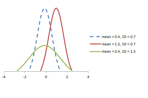
The mean µ is the parameter of this distribution. µ is also defined as the λ times length of that interval. The graph of a Poisson distribution is shown below:

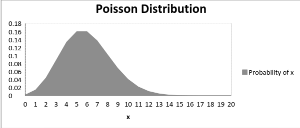
The graph shown below illustrates the shift in the curve due to increase in mean.

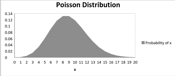
It is perceptible that as the mean increases, the curve shifts to the right.

The mean and variance of X following a Poisson distribution:

Mean -> E(X) = µ
Variance -> Var(X) = µ

Normal Distribution

Normal distribution represents the behavior of most of the situations in the universe (That is why it’s called a “normal” distribution. I guess!). The large sum of (small) random variables often turns out to be normally distributed, contributing to its widespread application. Any distribution is known as Normal distribution if it has the following characteristics:

1. The mean, median and mode of the distribution coincide.
2. The curve of the distribution is bell-shaped and symmetrical about the line x=μ.
3. The total area under the curve is 1.
4. Exactly half of the values are to the left of the center and the other half to the right.

A normal distribution is highly different from Binomial Distribution. However, if the number of trials approaches infinity then the shapes will be quite similar.

The PDF of a random variable X following a normal distribution is given by:

The mean and variance of a random variable X which is said to be normally distributed is given by:

Mean -> E(X) = µ

Variance -> Var(X) = σ^2

Here, µ (mean) and σ (standard deviation) are the parameters.
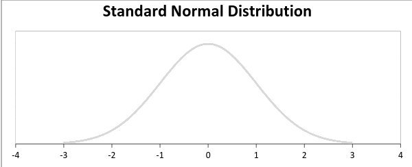
The graph of a random variable X ~ N (µ, σ) is shown below.

A standard normal distribution is defined as the distribution with mean 0 and standard deviation 1.  For such a case, the PDF becomes:

Binomial Distribution

Let’s get back to cricket.  Suppose that you won the toss today and this indicates a successful event. You toss again but you lost this time. If you win a toss today, this does not necessitate that you will win the toss tomorrow. Let’s assign a random variable, say X, to the number of times you won the toss. What can be the possible value of X? It can be any number depending on the number of times you tossed a coin.

There are only two possible outcomes. Head denoting success and tail denoting failure. Therefore, probability of getting a head = 0.5 and the probability of failure can be easily computed as: q = 1- p = 0.5.

A distribution where only two outcomes are possible, such as success or failure, gain or loss, win or lose and where the probability of success and failure is same for all the trials is called a Binomial Distribution.

The outcomes need not be equally likely. Remember the example of a fight between me and Undertaker? So, if the probability of success in an experiment is 0.2 then the probability of failure can be easily computed as q = 1 – 0.2 = 0.8.

Each trial is independent since the outcome of the previous toss doesn’t determine or affect the outcome of the current toss. An experiment with only two possible outcomes repeated n number of times is called binomial. The parameters of a binomial distribution are n and p where n is the total number of trials and p is the probability of success in each trial.

On the basis of the above explanation, the properties of a Binomial Distribution are

1. Each trial is independent.
2. There are only two possible outcomes in a trial- either a success or a failure.
3. A total number of n identical trials are conducted.
4. The probability of success and failure is same for all trials. (Trials are identical.)

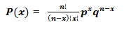
The mathematical representation of binomial distribution is given by:

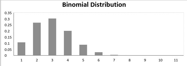
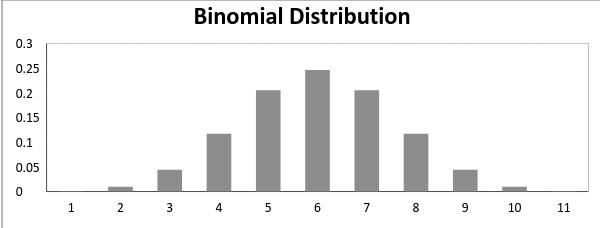
A binomial distribution graph where the probability of success does not equal the probability of failure looks like

Now, when probability of success = probability of failure, in such a situation the graph of binomial distribution looks like

The mean and variance of a binomial distribution are given by:

Mean -> µ = n*p

Variance -> Var(X) = n*p*q

Uniform Distribution

When you roll a fair die, the outcomes are 1 to 6. The probabilities of getting these outcomes are equally likely and that is the basis of a uniform distribution. Unlike Bernoulli Distribution, all the n number of possible outcomes of a uniform distribution are equally likely.

A variable X is said to be uniformly distributed if the density function is:

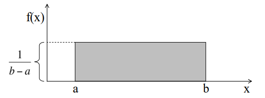
The graph of a uniform distribution curve looks like

You can see that the shape of the Uniform distribution curve is rectangular, the reason why Uniform distribution is called rectangular distribution.

For a Uniform Distribution, a and b are the parameters. 

The number of bouquets sold daily at a flower shop is uniformly distributed with a maximum of 40 and a minimum of 10.

Let’s try calculating the probability that the daily sales will fall between 15 and 30.

The probability that daily sales will fall between 15 and 30 is (30-15)*(1/(40-10)) = 0.5

Similarly, the probability that daily sales are greater than 20 is  = 0.667

The mean and variance of X following a uniform distribution is:

Mean -> E(X) = (a+b)/2

Variance -> V(X) =  (b-a)²/12

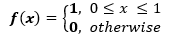
The standard uniform density has parameters a = 0 and b = 1, so the PDF for standard uniform density is given by:

Bernoulli Distribution

Let’s start with the easiest distribution that is Bernoulli Distribution. It is actually easier to understand than it sounds!

All you cricket junkies out there! At the beginning of any cricket match, how do you decide who is going to bat or ball? A toss! It all depends on whether you win or lose the toss, right? Let’s say if the toss results in a head, you win. Else, you lose. There’s no midway.

A Bernoulli distribution has only two possible outcomes, namely 1 (success) and 0 (failure), and a single trial. So the random variable X which has a Bernoulli distribution can take value 1 with the probability of success, say p, and the value 0 with the probability of failure, say q or 1-p.

Here, the occurrence of a head denotes success, and the occurrence of a tail denotes failure.
Probability of getting a head = 0.5 = Probability of getting a tail since there are only two possible outcomes.

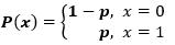
The probability mass function is given by: p^x(1-p)^1-x  where x € (0, 1).
It can also be written as

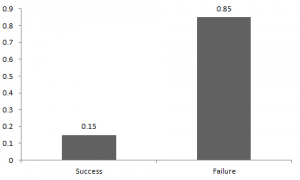
The probabilities of success and failure need not be equally likely, like the result of a fight between me and Undertaker. He is pretty much certain to win. So in this case probability of my success is 0.15 while my failure is 0.85

Here, the probability of success(p) is not same as the probability of failure. So, the chart below shows the Bernoulli Distribution of our fight.

Here, the probability of success = 0.15 and probability of failure = 0.85. The expected value is exactly what it sounds. If I punch you, I may expect you to punch me back. Basically expected value of any distribution is the mean of the distribution. The expected value of a random variable X from a Bernoulli distribution is found as follows:

E(X) = 1*p + 0*(1-p) = p

The variance of a random variable from a Bernoulli distribution is:

V(X) = E(X²) – [E(X)]² = p – p² = p(1-p)

There are many examples of Bernoulli distribution such as whether it’s going to rain tomorrow or not where rain denotes success and no rain denotes failure and Winning (success) or losing (failure) the game.

Tempo

Modalidades linguísticas

Comparações sobre fala e escrita

Funções da Linguagem

Configuring SQL Server 2008R2 Reporting Services Email Delivery with Gmail SMTP

his is how you can configure SQL Server 2008R2 Reporting Services email with Gmail SMTP server. Please note that my operating system is Windows Server 2008R2.

1. Go to Server Manager and Add feature “SMTP Server”. 
   

   

   Add Feature SMTP Server

2. Go to Administrative Tools and open Internet Information Services (IIS) 6.0 Manager.
3. Right Click on SMTP Virtual Server and select Properties.
   

   

   SMTP server properties

4. Under the General tab select your IP Address.
   

   

   IP Address

5. Under the Access tab click on Relay and do as follows.
   

   

   Relay

6. Under the Delivery tab you will get something like this.
   

   

   Delivery Tab

7. Now under the Delivery tab click on Outbound Security and type your gmail email address and the password. Remember to tick on "TLS encryption".
   

   

   Outbound Security

8. Again under the Delivery tab click on Outbound Connections and do as follows.
   

   

   Outbound Connections

9. Again under the Delivery tab click on Advanced and fill values as below.
   

   

   Advanced

10. Now you are done with the SMTP properties. Now make sure SMTP Server is started.
    

    

    Start SMTP Server

11. Go to Reporting Services Configuration Manager under Configuration Tools in All Program's Microsoft SQL Server 2008 R2. As Sender address, type your gmail address and as SMTP Server, type your IP address.
    

    

    Reporting Services Configuration Manager

12. Go to "C:\Program Files\Microsoft SQL Server\MSRS10_50.MSSQLSERVER\Reporting Services\ReportServer" and open "rsreportserver.config" file. Make sure your Report Manager URL is inside UrlRoot tags and Report Server Email Extension tag is filled as below with your details. If you find your tags empty, make a backup of "rsreportserver.config" file and fill the tag values as below.

            <UrlRoot>http://jaliya-pc/ReportServer</UrlRoot>

------------------------------------------------------------------------------------------------

            <Extension Name="Report Server Email" Type="Microsoft.ReportingServices.EmailDeliveryProvider.EmailProvider,ReportingServicesEmailDeliveryProvider">
                <MaxRetries>3</MaxRetries>
                <SecondsBeforeRetry>900</SecondsBeforeRetry>
                <Configuration>
                    <RSEmailDPConfiguration>
                        <SMTPServer>192.168.10.107</SMTPServer>
                        <SMTPServerPort>
                        </SMTPServerPort>
                        <SMTPAccountName>
                        </SMTPAccountName>
                        <SMTPConnectionTimeout>
                        </SMTPConnectionTimeout>
                        <SMTPServerPickupDirectory>
                        </SMTPServerPickupDirectory>
                        <SMTPUseSSL>
                        </SMTPUseSSL>
                        <SendUsing>2</SendUsing>
                        <SMTPAuthenticate>
                        </SMTPAuthenticate>
                        <From>jaliya.udagedara@gmail.com</From>
                        <EmbeddedRenderFormats>
                            <RenderingExtension>PDF</RenderingExtension>
                        </EmbeddedRenderFormats>
                        <PrivilegedUserRenderFormats>
                        </PrivilegedUserRenderFormats>
                        <ExcludedRenderFormats>
                            <RenderingExtension>HTMLOWC</RenderingExtension>
                            <RenderingExtension>NULL</RenderingExtension>
                            <RenderingExtension>RGDI</RenderingExtension>
                        </ExcludedRenderFormats>
                        <SendEmailToUserAlias>True</SendEmailToUserAlias>
                        <DefaultHostName>
                        </DefaultHostName>
                        <PermittedHosts>
                        </PermittedHosts>
                    </RSEmailDPConfiguration>
                </Configuration>
            </Extension>

------------------------------------------------------------------------------------------------

That's it. Now you can test your email delivery by creating a Data-driven Subscription. You can find the Reporting services log file under the following location. It will contain all the logs related to this email sending.

"C:\Program Files\Microsoft SQL Server\MSRS10_50.MSSQLSERVER\Reporting Services\LogFiles"

I am hoping to write a post about programmatically creating a Data-driven Subscription in a coming post and hope this helps.

Happy Coding.

Regards,

Jaliya

 http://jaliyaudagedara.blogspot.com/2012/09/configuring-sql-server-2008r2-reporting.html

 

Anxiety

Distúrbio de Percepção

Uma crônica tentativa de antecipação de eventos futuros que desencadeavam respostas para situações que, provavelmente, não aconteceriam. Essas respostas, geralmente, estavam acima das capacidades atuais. Isso ocasionava um nível de stress que acabou consumindo grande parte do processamento do cérebro e fez com que questões importantes ou do dia-a-dia ficassem de lado. Além disso, essas respostas aumentavam a irritabilidade, o senso de perseguição, rejeição, angústia e a percepção exagerada de problemas triviais.

Activation Functions

Recommender Systems Evaluation

Activation Functions