Binomial Distribution

Let’s get back to cricket.  Suppose that you won the toss today and this indicates a successful event. You toss again but you lost this time. If you win a toss today, this does not necessitate that you will win the toss tomorrow. Let’s assign a random variable, say X, to the number of times you won the toss. What can be the possible value of X? It can be any number depending on the number of times you tossed a coin.

There are only two possible outcomes. Head denoting success and tail denoting failure. Therefore, probability of getting a head = 0.5 and the probability of failure can be easily computed as: q = 1- p = 0.5.

A distribution where only two outcomes are possible, such as success or failure, gain or loss, win or lose and where the probability of success and failure is same for all the trials is called a Binomial Distribution.

The outcomes need not be equally likely. Remember the example of a fight between me and Undertaker? So, if the probability of success in an experiment is 0.2 then the probability of failure can be easily computed as q = 1 – 0.2 = 0.8.

Each trial is independent since the outcome of the previous toss doesn’t determine or affect the outcome of the current toss. An experiment with only two possible outcomes repeated n number of times is called binomial. The parameters of a binomial distribution are n and p where n is the total number of trials and p is the probability of success in each trial.

On the basis of the above explanation, the properties of a Binomial Distribution are

1. Each trial is independent.
2. There are only two possible outcomes in a trial- either a success or a failure.
3. A total number of n identical trials are conducted.
4. The probability of success and failure is same for all trials. (Trials are identical.)

The mathematical representation of binomial distribution is given by:

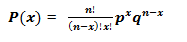
A binomial distribution graph where the probability of success does not equal the probability of failure looks like

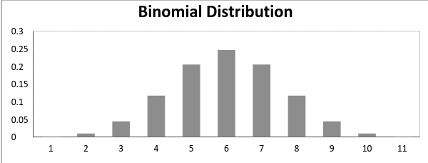
Now, when probability of success = probability of failure, in such a situation the graph of binomial distribution looks like

The mean and variance of a binomial distribution are given by:

Mean -> µ = n*p

Variance -> Var(X) = n*p*q