It's Just A Ride - Bill Hicks

The Ptolemaic Universe, in which complex motion of the planets in the night sky was explained by orbits within orbits, called epicycles. The model is incredibly wrong, yet makes quite good predictions.

 

Probability vs. Likelihood

 

Risk Exposure

 

Selecting an appropriate statistical procedure

 

Hypotheses are not models

 

Relations among hypotheses (left), detailed process models (middle), and statistical models (right), illustrated by the example of “neutral” models of evolution. Hypotheses (H) are typically vague, and so correspond to more than one process model (P). Statistical evaluations of hypotheses rarely address process models directly. Instead, they rely upon statistical models (M), all of which reflect only some aspects of the process models. As a result, relations are multiple in both directions: Hypotheses do not imply unique models, and models do not imply unique hypotheses. This fact greatly complicates statistical inference.

Heteroscedasticidade

 

Characterizing a Distribution

 

Probability Distribution

 

Kepler's second law

 

Torus

 

DataSaurus

 

Interpolation

 

Bloom

 

Bloom

 

Bloom

 

Composite Functions

 

Logarithmic Functions

 

Graphs of the sine and cosine functions

 

To graph the function y = ƒ(x) shown here, we apply different formulas to different parts of its domain

 

Graphs of ƒ(x) = x^n, n = 1, 2, 3, 4, 5, defined for -q 6 x 6 q.

 

Let me not seem to have lived in vain.

 

It shouldn't bother me... It shouldn't, but it does

 

The domains in each case are the values of x for which the formula makes sense.

 

Functions

 

Cérebro

 

The Architecture of Sleep

 

Gravitacional Tides on Black Holes

 

The Earth’s habitable zone, defined as the region around the Sun where water could be found in liquid form. Therefore, if there is a planet suitable for supporting life (as we know based on our definition of life), it must reside within the habitable zone of its star. The Earth is in the habitable zone of the Sun.

 

Schematic picture showing the increase in the size of a low-mass star as a result of fuel burning at the core and shifting of the hydrogen- and helium-burning layers to larger radii. Eventually, the outer envelope of the star is ejected, forming a planetary nebula. Different colors in the planetary nebula indicate sites of different chemical elements.

 

The development of complex living things, from a cell to more complicated systems

 

Shows different stages in the evolution of a low-mass star (top) and massive star (bottom)

 

Characteristics of the fundamental forces in the universe

 

Regras de aquisição Ferengis

No universo de Jornada nas Estrelas, uma das espécies que apresentam mais curiosidade são os Ferengis, principalmente no que se diz respeito nas suas "Regras de Aquisição".[2]

Podem ser descritas como uma espécie de Bíblia para os Ferengis e todos os machos adultos da espécie são obrigados a recita-las de cor.

As principais regras

1ª regra: "Uma vez que você tenha o dinheiro deles, nunca devolva".

3ª regra: "Nunca gaste mais em uma aquisição do que necessário".

6ª regra: "Nunca permita que a família fique no caminho da oportunidade".

7ª regra: "Mantenha suas orelhas abertas".

9ª regra: "Oportunidade mais instinto é igual a lucro".

10ª regra: "Ambição é eterna".

16ª regra: "Um trato é um trato".

17ª regra: "Um contrato é um contrato - mas somente entre ferengis".

18ª regra: "Um ferengi sem lucro não é ferengi de qualquer maneira".

19ª regra: "Satisfação não garantida".

21ª regra: "Nunca ponha a amizade acima do lucro".

22ª regra: "Um homem experiente pode ouvir lucro no vento".

23ª regra: "Nunca tire a última moeda de alguém, mas tenha certeza de ter tirado o resto".

31ª regra: "Nunca ofenda a mãe de um ferengi... insulte algo que ele se importe ao invés".

33ª regra: "Não custa puxar o saco do chefe".

34ª regra: "A guerra é boa para os negócios".

35ª regra: "A paz é boa para os negócios".

45ª regra: "Expanda ou morra - Um homem só vale a soma dos seus bens".

47ª regra: "Nunca confie em alguém cuja roupa é melhor que a sua própria".

49ª regra: "Quanto maior for o sorriso, mais afiada será a faca".

57ª regra: "Bons consumidores são como ouro latinum. Valorize-os".

59ª regra: "Conselho de graça quase nunca é barato".

62ª regra: "Quanto mais risco tiver o caminho, maior será o lucro".

74ª regra: "Conhecimento é igual ao lucro".

75ª regra: "Lar é onde o coração está, mas as estrelas são feitas de ouro latinum".

76ª regra: "De vez em quando, declare a paz. Isso confunde seus inimigos".

94ª regra: "Mulheres e finanças não se misturam".

98ª regra: "Todo homem tem seu preço".

102ª regra: "A Natureza decai, mas ouro latinum é para sempre".

109ª regra: "Entre dignidade e um saco vazio, fique com o saco".

111ª regra: "Trate pessoas em dívida como a sua família - explore-os".

112ª regra: "Nunca faça sexo com a irmã do chefe".

125ª regra: "Você não pode fazer negócios se você estiver morto".

139ª regra: "Esposas servem. Irmãos herdam".

168ª regra Sussurre seu caminho para o sucesso

190ª regra: "Ouça tudo e não creia em nada."

194ª regra: "É sempre bom conhecer seus novos consumidores antes que eles entrem pela sua porta".

199ª regra: "Um ferengi sem lucro não é ferengi nenhum".

203ª regra: "Novos consumidores são como razor-backed Greeworms (uma iguaria para os Ferengis) - podem ser suculentos, mas às vezes mordem de volta!".

208ª regra: "As vezes a única coisa mais perigosa que uma pergunta é uma resposta".

211ª regra: "Empregados são os degraus da escada do sucesso - não hesite em pisar sobre eles".

214ª regra: "Nunca comece a negociar com o estômago vazio".

217ª regra: "Você não pode libertar um peixe da água". (Não se pode "endireitar" um Ferengi).

223ª regra: "Ouro latinum dura mais que a luxúria".

229ª regra: "Latinum dura mais que paixão".

239ª regra: "Não tenha medo de nomear um produto erroneamente".

263ª regra: "Nunca permita que a dúvida diminua seu desejo por latinum".

285ª regra: "Nenhuma boa proeza fica impune". (Fazer caridade é uma das piores ofensas para um Ferengi - principalmente com o dinheiro deles).

Typing

 

THE MACHINE LEARNING PROCESS

• Data Collection and Preparation. Throughout this book we will be in the fortunate position of having datasets readily available for downloading and using to test the algorithms. This is, of course, less commonly the case when the desire is to learn about some new problem, when either the data has to be collected from scratch, or at the very least, assembled and prepared. In fact, if the problem is completely new, so that appropriate data can be chosen, then this process should be merged with the next step of feature selection, so that only the required data is collected. This can typically be done by assembling a reasonably small dataset with all of the features that you believe might be useful, and experimenting with it before choosing the best features and collecting and analysing the full dataset. Often the difficulty is that there is a large amount of data that might be relevant, but it is hard to collect, either because it requires many measurements to be taken, or because they are in a variety of places and formats, and merging it appropriately is difficult, as is ensuring that it is clean; that is, it does not have significant errors, missing data, etc. For supervised learning, target data is also needed, which can require the involvement of experts in the relevant field and significant investments of time. Finally, the quantity of data needs to be considered. Machine learning algorithms need significant amounts of data, preferably without too much noise, but with increased dataset size comes increased computational costs, and the sweet spot at which there is enough data without excessive computational overhead is generally impossible to predict. 

• Feature Selection. An example of this part of the process was given in Section 1.4.2 when we looked at possible features that might be useful for coin recognition. It consists of identifying the features that are most useful for the problem under examination. This invariably requires prior knowledge of the problem and the data; our common sense was used in the coins example above to identify some potentially useful features and to exclude others. As well as the identification of features that are useful for the learner, it is also necessary that the features can be collected without significant expense or time, and that they are robust to noise and other corruption of the data that may arise in the collection process.

• Algorithm Choice. Given the dataset, the choice of an appropriate algorithm (or algorithms) is what this book should be able to prepare you for, in that the knowledge of the underlying principles of each algorithm and examples of their use is precisely what is required for this.

• Parameter and Model Selection. For many of the algorithms there are parameters that have to be set manually, or that require experimentation to identify appropriate values. These requirements are discussed at the appropriate points of the book.

• Training Given. the dataset, algorithm, and parameters, training should be simply the use of computational resources in order to build a model of the data in order to predict the outputs on new data.

• Evaluation. Before a system can be deployed it needs to be tested and evaluated for accuracy on data that it was not trained on. This can often include a comparison with human experts in the field, and the selection of appropriate metrics for this comparison.

Some counts and measures for the hype

 

The Curse of Dimensionality in classification

 

Introduction

In this article, we will discuss the so called ‘Curse of Dimensionality’, and explain why it is important when designing a classifier. In the following sections I will provide an intuitive explanation of this concept, illustrated by a clear example of overfitting due to the curse of dimensionality.

Consider an example in which we have a set of images, each of which depicts either a cat or a dog. We would like to create a classifier that is able to distinguish dogs from cats automatically. To do so, we first need to think about a descriptor for each object class that can be expressed by numbers, such that a mathematical algorithm, i.e. a classifier, can use these numbers to recognize the object. We could for instance argue that cats and dogs generally differ in color. A possible descriptor that discriminates these two classes could then consist of three number; the average red color, the average green color and the average blue color of the image under consideration. A simple linear classifier for instance, could combine these features linearly to decide on the class label:

If 0.5*red + 0.3*green + 0.2*blue > 0.6 : return cat;
else return dog;

However, these three color-describing numbers, called features, will obviously not suffice to obtain a perfect classification. Therefore, we could decide to add some features that describe the texture of the image, for instance by calculating the average edge or gradient intensity in both the X and Y direction. We now have 5 features that, in combination, could possibly be used by a classification algorithm to distinguish cats from dogs.

To obtain an even more accurate classification, we could add more features, based on color or texture histograms, statistical moments, etc. Maybe we can obtain a perfect classification by carefully defining a few hundred of these features? The answer to this question might sound a bit counter-intuitive: no we can not!. In fact, after a certain point, increasing the dimensionality of the problem by adding new features would actually degrade the performance of our classifier. This is illustrated by figure 1, and is often referred to as ‘The Curse of Dimensionality’.

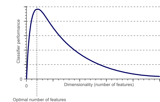
Figure 1. As the dimensionality increases, the classifier’s performance increases until the optimal number of features is reached. Further increasing the dimensionality without increasing the number of training samples results in a decrease in classifier performance.

In the next sections we will review why the above is true, and how the curse of dimensionality can be avoided.

The curse of dimensionality and overfitting

In the earlier introduced example of cats and dogs, let’s assume there are an infinite number of cats and dogs living on our planet. However, due to our limited time and processing power, we were only able to obtain 10 pictures of cats and dogs. The end-goal in classification is then to train a classifier based on these 10 training instances, that is able to correctly classify the infinite number of dog and cat instances which we do not have any information about.

Now let’s use a simple linear classifier and try to obtain a perfect classification. We can start by a single feature, e.g. the average ‘red’ color in the image:

Figure 2. A single feature does not result in a perfect separation of our training data.

Figure 2 shows that we do not obtain a perfect classification result if only a single feature is used. Therefore, we might decide to add another feature, e.g. the average ‘green’ color in the image:

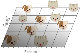
Figure 3.Adding a second feature still does not result in a linearly separable classification problem: No single line can separate all cats from all dogs in this example.

Finally we decide to add a third feature, e.g. the average ‘blue’ color in the image, yielding a three-dimensional feature space:

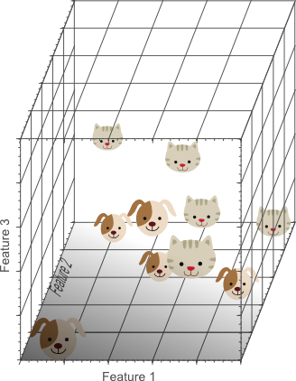
Figure 4. Adding a third feature results in a linearly separable classification problem in our example. A plane exists that perfectly separates dogs from cats.

In the three-dimensional feature space, we can now find a plane that perfectly separates dogs from cats. This means that a linear combination of the three features can be used to obtain perfect classification results on our training data of 10 images:

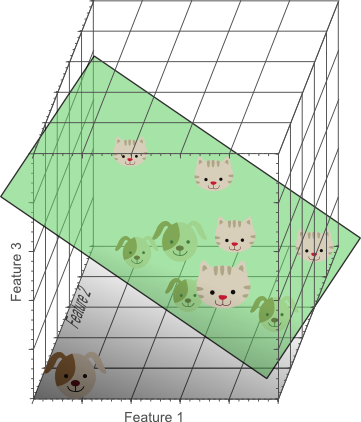
Figure 5. The more features we use, the higher the likelihood that we can successfully separate the classes perfectly.

The above illustrations might seem to suggest that increasing the number of features until perfect classification results are obtained is the best way to train a classifier, whereas in the introduction, illustrated by figure 1, we argued that this is not the case. However, note how the density of the training samples decreased exponentially when we increased the dimensionality of the problem.

In the 1D case (figure 2), 10 training instances covered the complete 1D feature space, the width of which was 5 unit intervals. Therefore, in the 1D case, the sample density was 10/5=2 samples/interval. In the 2D case however (figure 3), we still had 10 training instances at our disposal, which now cover a 2D feature space with an area of 5×5=25 unit squares. Therefore, in the 2D case, the sample density was 10/25 = 0.4 samples/interval. Finally, in the 3D case, the 10 samples had to cover a feature space volume of 5x5x5=125 unit cubes. Therefore, in the 3D case, the sample density was 10/125 = 0.08 samples/interval.

If we would keep adding features, the dimensionality of the feature space grows, and becomes sparser and sparser. Due to this sparsity, it becomes much more easy to find a separable hyperplane because the likelihood that a training sample lies on the wrong side of the best hyperplane becomes infinitely small when the number of features becomes infinitely large. However, if we project the highly dimensional classification result back to a lower dimensional space, a serious problem associated with this approach becomes evident:

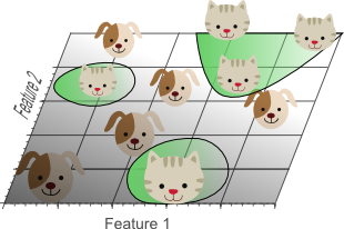
Figure 6. Using too many features results in overfitting. The classifier starts learning exceptions that are specific to the training data and do not generalize well when new data is encountered.

Figure 6 shows the 3D classification results, projected onto a 2D feature space. Whereas the data was linearly separable in the 3D space, this is not the case in a lower dimensional feature space. In fact, adding the third dimension to obtain perfect classification results, simply corresponds to using a complicated non-linear classifier in the lower dimensional feature space. As a result, the classifier learns the appearance of specific instances and exceptions of our training dataset. Because of this, the resulting classifier would fail on real-world data, consisting of an infinite amount of unseen cats and dogs that often do not adhere to these exceptions.

This concept is called overfitting and is a direct result of the curse of dimensionality. Figure 7 shows the result of a linear classifier that has been trained using only 2 features instead of 3:

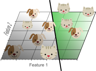
Figure 7. Although the training data is not classified perfectly, this classifier achieves better results on unseen data than the one from figure 5.

Although the simple linear classifier with decision boundaries shown by figure 7 seems to perform worse than the non-linear classifier in figure 5, this simple classifier generalizes much better to unseen data because it did not learn specific exceptions that were only in our training data by coincidence. In other words, by using less features, the curse of dimensionality was avoided such that the classifier did not overfit the training data.

Figure 8 illustrates the above in a different manner. Let’s say we want to train a classifier using only a single feature whose value ranges from 0 to 1. Let’s assume that this feature is unique for each cat and dog. If we want our training data to cover 20% of this range, then the amount of training data needed is 20% of the complete population of cats and dogs. Now, if we add another feature, resulting in a 2D feature space, things change; To cover 20% of the 2D feature range, we now need to obtain 45% of the complete population of cats and dogs in each dimension (0.45^2 = 0.2). In the 3D case this gets even worse: to cover 20% of the 3D feature range, we need to obtain 58% of the population in each dimension (0.58^3 = 0.2).

Figure 8. The amount of training data needed to cover 20% of the feature range grows exponentially with the number of dimensions.

In other words, if the amount of available training data is fixed, then overfitting occurs if we keep adding dimensions. On the other hand, if we keep adding dimensions, the amount of training data needs to grow exponentially fast to maintain the same coverage and to avoid overfitting.

In the above example, we showed that the curse of dimensionality introduces sparseness of the training data. The more features we use, the more sparse the data becomes such that accurate estimation of the classifier’s parameters (i.e. its decision boundaries) becomes more difficult. Another effect of the curse of dimensionality, is that this sparseness is not uniformly distributed over the search space. In fact, data around the origin (at the center of the hypercube) is much more sparse than data in the corners of the search space. This can be understood as follows:

Imagine a unit square that represents the 2D feature space. The average of the feature space is the center of this unit square, and all points within unit distance from this center, are inside a unit circle that inscribes the unit square. The training samples that do not fall within this unit circle are closer to the corners of the search space than to its center. These samples are difficult to classify because their feature values greatly differs (e.g. samples in opposite corners of the unit square). Therefore, classification is easier if most samples fall inside the inscribed unit circle, illustrated by figure 9:

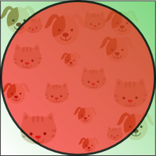
Figure 9.Training samples that fall outside the unit circle are in the corners of the feature space and are more difficult to classify than samples near the center of the feature space.

An interesting question is now how the volume of the circle (hypersphere) changes relative to the volume of the square (hypercube) when we increase the dimensionality of the feature space. The volume of a unit hypercube of dimension d is always 1^d = 1. The volume of the inscribing hypersphere of dimension d and with radius 0.5 can be calculated as:

(1) 

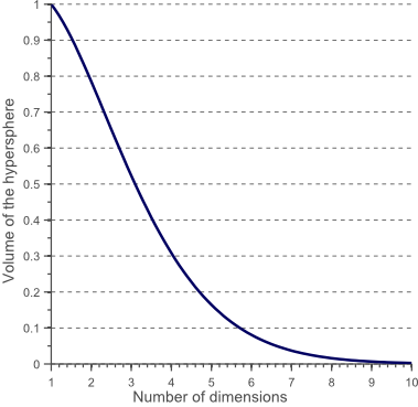
Figure 10 shows how the volume of this hypersphere changes when the dimensionality increases:

Figure 10. The volume of the hypersphere tends to zero as the dimensionality increases.

This shows that the volume of the hypersphere tends to zero as the dimensionality tends to infinity, whereas the volume of the surrounding hypercube remains constant. This surprising and rather counter-intuitive observation partially explains the problems associated with the curse of dimensionality in classification: In high dimensional spaces, most of the training data resides in the corners of the hypercube defining the feature space. As mentioned before, instances in the corners of the feature space are much more difficult to classify than instances around the centroid of the hypersphere. This is illustrated by figure 11, which shows a 2D unit square, a 3D unit cube, and a creative visualization of an 8D hypercube which has 2^8 = 256 corners:

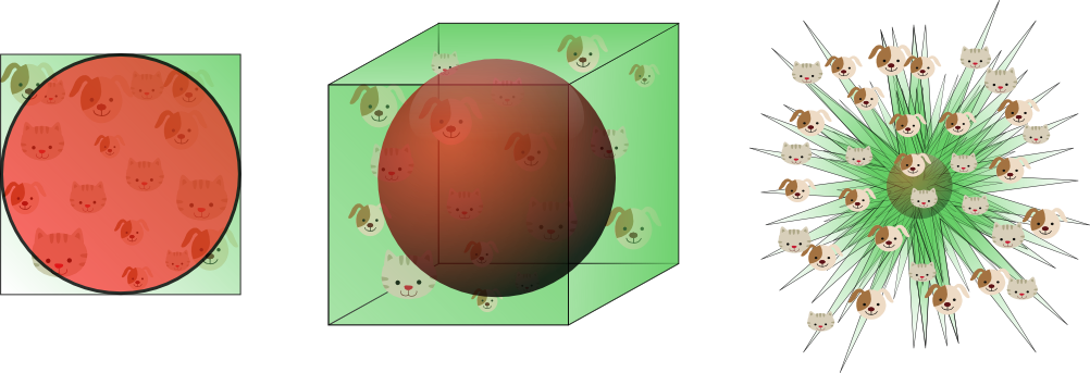
Figure 11. As the dimensionality increases, a larger percentage of the training data resides in the corners of the feature space.

For an 8-dimensional hypercube, about 98% of the data is concentrated in its 256 corners. As a result, when the dimensionality of the feature space goes to infinity, the ratio of the difference in minimum and maximum Euclidean distance from sample point to the centroid, and the minimum distance itself, tends to zero:

(2) 

Therefore, distance measures start losing their effectiveness to measure dissimilarity in highly dimensional spaces. Since classifiers depend on these distance measures (e.g. Euclidean distance, Mahalanobis distance, Manhattan distance), classification is often easier in lower-dimensional spaces where less features are used to describe the object of interest. Similarly, Gaussian likelihoods become flat and heavy tailed distributions in high dimensional spaces, such that the ratio of the difference between the minimum and maximum likelihood and the minimum likelihood itself tends to zero.

How to avoid the curse of dimensionality?

Figure 1 showed that the performance of a classifier decreases when the dimensionality of the problem becomes too large. The question then is what ‘too large’ means, and how overfitting can be avoided. Regrettably there is no fixed rule that defines how many feature should be used in a classification problem. In fact, this depends on the amount of training data available, the complexity of the decision boundaries, and the type of classifier used.

If the theoretical infinite number of training samples would be available, the curse of dimensionality does not apply and we could simply use an infinite number of features to obtain perfect classification. The smaller the size of the training data, the less features should be used. If N training samples suffice to cover a 1D feature space of unit interval size, then N^2 samples are needed to cover a 2D feature space with the same density, and N^3 samples are needed in a 3D feature space. In other words, the number of training instances needed grows exponentially with the number of dimensions used.

Furthermore, classifiers that tend to model non-linear decision boundaries very accurately (e.g. neural networks, KNN classifiers, decision trees) do not generalize well and are prone to overfitting. Therefore, the dimensionality should be kept relatively low when these classifiers are used. If a classifier is used that generalizes easily (e.g. naive Bayesian, linear classifier), then the number of used features can be higher since the classifier itself is less expressive. Figure 6 showed that using a simple classifier model in a high dimensional space corresponds to using a complex classifier model in a lower dimensional space.

Therefore, overfitting occurs both when estimating relatively few parameters in a highly dimensional space, and when estimating a lot of parameters in a lower dimensional space. As an example, consider a Gaussian density function, parameterized by its mean and covariance matrix. Let’s say we operate in a 3D space, such that the covariance matrix is a 3×3 symmetric matrix consisting of 6 unique elements (3 variances on the diagonal and 3 covariances off-diagonal). Together with the 3D mean of the distribution this means that we need to estimate 9 parameters based on our training data, to obtain the Gaussian density that represent the likelihood of our data. In the 1D case, only 2 parameters need to be estimated (mean and variance), whereas in the 2D case 5 parameters are needed (2D mean, two variances and a covariance). Again we can see that the number of parameters to be estimated grows quadratic with the number of dimensions.

In an earlier article we showed that the variance of a parameter estimate increases if the number of parameters to be estimated increases (and if the bias of the estimate and the amount of training data are kept constant). This means that the quality of our parameter estimates decreases if the dimensionality goes up, due to the increase of variance. An increase of classifier variance corresponds to overfitting.

Another interesting question is which features should be used. Given a set of N features; how do we select an optimal subset of M features such that M<N? One approach would be to search for the optimum in the curve shown by figure 1. Since it is often intractable to train and test classifiers for all possible combinations of all features, several methods exist that try to find this optimum in different manners. These methods are called feature selection algorithms and often employ heuristics (greedy methods, best-first methods, etc.) to locate the optimal number and combination of features.

Another approach would be to replace the set of N features by a set of M features, each of which is a combination of the original feature values. Algorithms that try to find the optimal linear or non-linear combination of original features to reduce the dimensionality of the final problem are called Feature Extraction methods. A well known dimensionality reduction technique that yields uncorrelated, linear combinations of the original N features is Principal Component Analysis (PCA). PCA tries to find a linear subspace of lower dimensionality, such that the largest variance of the original data is kept. However, note that the largest variance of the data not necessarily represents the most discriminative information.

Finally, an invaluable technique used to detect and avoid overfitting during classifier training is cross-validation. Cross validation approaches split the original training data into one or more training subsets. During classifier training, one subset is used to test the accuracy and precision of the resulting classifier, while the others are used for parameter estimation. If the classification results on the subsets used for training greatly differ from the results on the subset used for testing, overfitting is in play. Several types of cross-validation such as k-fold cross-validation and leave-one-out cross-validation can be used if only a limited amount of training data is available.

Conclusion

In this article we discussed the importance of feature selection, feature extraction, and cross-validation, in order to avoid overfitting due to the curse of dimensionality. Using a simple example, we reviewed an important effect of the curse of dimensionality in classifier training, namely overfitting.