Exponential Distribution

Let’s consider the call center example one more time. What about the interval of time between the calls ? Here, exponential distribution comes to our rescue. Exponential distribution models the interval of time between the calls.

Other examples are:

1. Length of time beteeen metro arrivals,
2. Length of time between arrivals at a gas station
3. The life of an Air Conditioner

Exponential distribution is widely used for survival analysis. From the expected life of a machine to the expected life of a human, exponential distribution successfully delivers the result.

A random variable X is said to have an exponential distribution with PDF:

f(x) = { λe^-λx,  x ≥ 0

and parameter λ>0 which is also called the rate.

For survival analysis, λ is called the failure rate of a device at any time t, given that it has survived up to t.

Mean and Variance of a random variable X following an exponential distribution:

Mean -> E(X) = 1/λ

Variance -> Var(X) = (1/λ)²

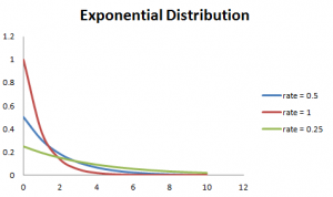
Also, the greater the rate, the faster the curve drops and the lower the rate, flatter the curve. This is explained better with the graph shown below.

To ease the computation, there are some formulas given below.
P{X≤x} = 1 – e^-λx, corresponds to the area under the density curve to the left of x.

P{X>x} = e^-λx, corresponds to the area under the density curve to the right of x.

P{x1-λx1

 – e^-λx2, corresponds to the area under the density curve between x1 and x2.